How To Add Multiple Data Labels In Excel Line Chart
Now click on Insert Tab from the top of the Excel window and then select Insert Line or Area Chart. This time click on the Add button on the left side of the dialog box.
Multiple Series In One Excel Chart Peltier Tech
Click any data label to select all data labels and then click the specified data label to select it only in the chart.

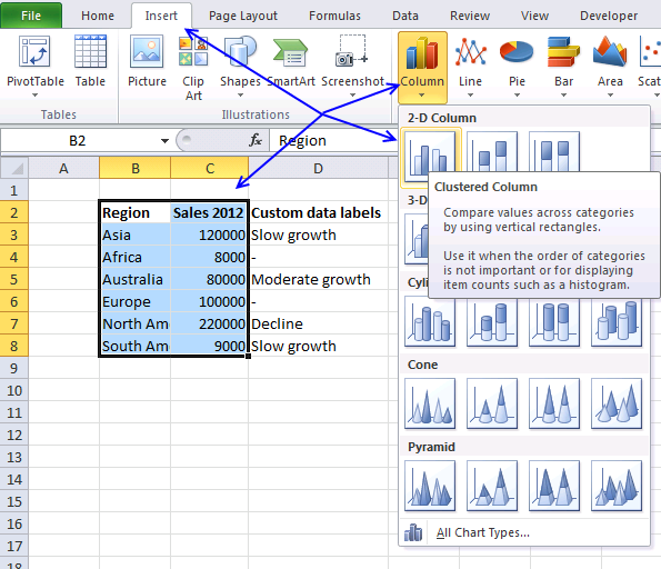
How to add multiple data labels in excel line chart. In this video Ill show you how to add data labels to a chart in Excel and then change the range that the data labels are linked to. If you have selected the entire data series you wont see this command. And select Clustered Bar chart type.
Make sure that you have selected just one data label. About Press Copyright Contact us Creators Advertise Developers Terms Privacy Policy Safety How YouTube works Test new features Press Copyright Contact us Creators. Click again on the single point that you want to add a data label to.
Select A1D4 and insert a bar chart. Apply data labels to series 2 outside end. To edit the series labels follow these steps.
Adjust series 2 data references Value from B2D2. Category labels from B4D4. Follow the below steps to implement the same.
The two data series are now shown combined as a. This brings up the dialog box shown in Figure 3 of Excel Line Charts. 2 go to INSERT tab click Bar command under charts group.
Only if you have numeric labels empty cell A1 before you create the line chart. If you have created a column chart you can select the item Data Edit data in the function bar and thus add a second data series. And you can do the following steps to add a vertical line to the horizontal bar chart type in Excel.
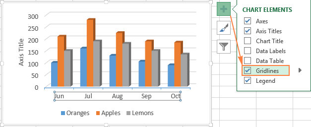
Select 2 series diff base line and move to secondary axis. Insert the data in the cells. Click the chart to show the Chart Elements button.
If you would only like to add a titlelabel for one axis horizontal or vertical click the right arrow beside Axis Titles and select which axis you would like to add a titlelabel. Right click the data series in the chart and select Add Data Labels Add Data Labels from the context menu to add data labels. Apply data labels to series 1 inside end.
Then check the tickbox for Axis Titles. In Example 1 the two columns of data Income and Rent are contiguous. You cant edit the Chart Data Range to include multiple blocks of data.
1 select the original data that you want to build a horizontal bar chart. Select 2 series and delete it. Now you can select the Line display under Type under the function bar via Colors and Style.
If they are not contiguous you could highlight. On the Design tab in the Chart Layouts group click Add Chart Element choose Data Labels and then click None. By doing this Excel does not recognize the numbers in column A as a data series and automatically places these numbers on the horizontal category axis.
Create the chart as usual Add default data labels Click on each unwanted label using slow double click and delete it Select each item where you want the custom label one at a time. After creating the chart you can enter the text Year into cell A1 if you like. However you can add data by clicking the Add button above the list of series which includes just the first series.
Click a data label one time to select all data labels in a data series or two times to select just one data label that you want to delete and then press DELETE. Click on the chart line to add the data point to. Right-click and select Add data label.
Right-click a data label. This video covers both W. Add titles and series labels Click on the chart to open the Chart Tools contextual tab then edit the Chart title by clicking on the Chart Title textbox.
Click Line with Markers. On the Insert tab in the Charts group click the Line symbol. In the dialog box that appears see Figure 3 enter Rent as the Series name and C4C13 as the series values and then click on the OK button.
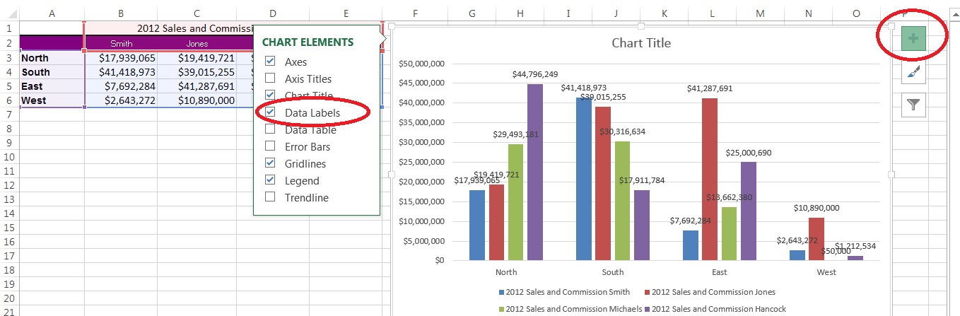
Then click the Chart Elements and check Data Labels then you can click the arrow to choose an option about the data labels in the sub menu. First off you have to click the chart and click the plus icon on the upper-right side. Right click the chart and choose Select Data or click on Select Data in the ribbon to bring up the Select Data Source dialog.
Select Series Data. From the pop-down menu select the first 2-D Line. After insertion select the rows and columns by dragging the cursor.
Click the data label right click it and then click Insert Data Label Field. All the data points will be highlighted. Verified 4 days ago.
Click Select Data button on the Design tab to open the Select Data Source dialog box.
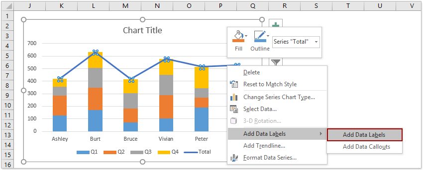
How To Add Total Labels To Stacked Column Chart In Excel
Quick Tip Excel 2013 Offers Flexible Data Labels Techrepublic

How To Use Data Labels From A Range In An Excel Chart Excel Dashboard Templates

Apply Custom Data Labels To Charted Points Peltier Tech

Adding Data Label Only To The Last Value Super User

How To Add Data Labels From Different Column In An Excel Chart
Custom Data Labels In A Chart

How To Add Data Labels From Different Column In An Excel Chart

How To Change Excel Chart Data Labels To Custom Values
Excel Charts Add Title Customize Chart Axis Legend And Data Labels

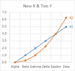
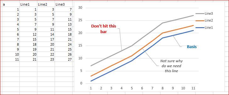
Dynamically Label Excel Chart Series Lines My Online Training Hub
How To Add Data Labels From Different Column In An Excel Chart

How To Add Data Labels To An Excel 2010 Chart Dummies

Excel Charts Add Title Customize Chart Axis Legend And Data Labels
How To Customize Your Excel Pivot Chart Data Labels Dummies

How To Add Data Labels From Different Column In An Excel Chart
Line Charts Moving The Legends Next To The Line Microsoft Tech Community

Two Level Axis Labels Microsoft Excel
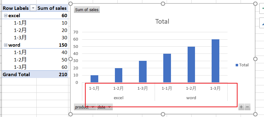
How To Create A Chart With Two Level Axis Labels In Excel Free Excel Tutorial