How To Put Negative Numbers In Excel Graph
Select the cells which have the negative percentage you want to mark in red. On the left choose the Number category.
How To Make An Excel Chart Go Up With Negative Values Excel Dashboard Templates
Right click the X axis in the chart and select the Format Axis from the right-clicking menu.
How to put negative numbers in excel graph. In the popping dialog choose one chart type you need the choose the axis labels two series values separately. Verify that negative numbers are added with brackets. To do this select the cell or range of cells to be formatted then if using Microsoft Excel 2003 or earlier click Format Cells and ensure the.
Then select All option from the Paste and Multiply from the Operation. 1 In Excel 2013s Format Axis pane expand the Labels on the Axis Options tab click the Label Position box and select Low from the drop down list. Next Ill right-click on any of the bars choose Format data series then click on the Fill Line option and put a check mark next to Invert if negative.
The number is -12 and the log of a negative number cannot be calculated. With the Positive Negative Bar Chart tool of Kutools for Excel which only needs 3 steps to deal with this job in Excel. Click Kutools Charts Positive Negative Bar Chart.
And if you source data have negative values and you want to move X Axis labels below negative how to achieve it. The first argument of the LN in Excel is B10 the number for which log is to be calculated. Navigate to the Home tab under the Excel ribbon and click on the small arrow type of icon which is there to enlarge the number formatting under the Number group.
Click Format Cells on menu. Put a check in the Error Bars checkbox. Select the series in your chart and press Ctrl1 to open the Format Series task pane.
And then click OK all of the positive numbers have. On the right choose an option from the Negative Numbers list and then hit OK Note that the image below shows the options youd see in the US. In the Format Cells window switch to the Number tab.
Now we will see how to represent the negative numbers with the built-in number formatting in Excel. Or by clicking on this icon in the ribbon Code to. Rather than having negative numbers with a minus sign in front of them some people prefer to put negative numbers in brackets.
Highlight the range that you want to change then right-click and choose Paste Special from the context menu to open. Move X Axis to Bottom for Negative Data. Since the value is negative the LN function in Excel returns an error indicating the value is erroneous.
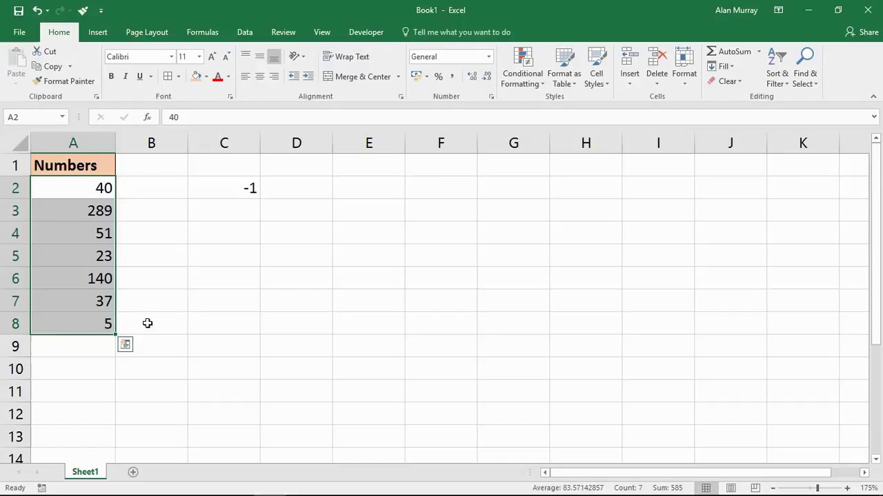
Select all the data from your cells as shown below. This excel chart is supposed to display negative numbers Profit. Tap number -1 in a blank cell and copy it.
Hey Guys I need your help. If you have Excel 2013 choose the Format Data Series from the right click menu to open the Format Data Series pane and then click Fill Line icon and check Invert if negative option then check Solid fill and specify the colors for the positive and negative data bar as you want beside Color section. On Format Cells under Number tab click Number in Category list then in Negative numbers list select number with brackets.
When you created a bar chart or line chart in your worksheet and the X Axis labels are stuck at 0 position of the Axis. Open the dialog box Format Cells using the shortcut Ctrl 1 or by clicking on the last option of the Number Format dropdown list. Select the positive color blue below using the Foreground paint can and the negative color orange using the Background paint can.
There is no positive or negative connotation in the format. First Ill just create a simple column chart from the data. Click on the chart then click the Chart Elements Button to open the fly-out list of checkboxes.
Then click OK to confirm update. And choose the Dotted 90 pattern. Notice how the bars for the negative values turned clear or transparent.
I formatted the values to be sure they are numbers didnt do anything. Click the arrow beside the Error Bars checkbox to choose from common error types. In fact any negative values are treated to the default treatment which is the third format.
You can create a custom format to quickly format all negative percentage in red in Excel. Go ahead based on your Microsoft Excels version. What you are trying to do is to define two positive conditions one for millions and one for thousands and two negative conditions again for millions and thousands.
But instead the Y-graph starts at 0 in the first place and the profit graph is displayed as being at value zero where it would be supposed to be negative. To display your negative numbers with parentheses we must create our own number format. Select Pattern Fill and Invert if Negative.

Replace Negative Values With Zero In Excel Google Sheets Automate Excel

Excel Formula Force Negative Numbers To Zero Exceljet
How To Prevent Excel Charts From Displaying Negative Numbers Quora
How To Make An Excel Chart Go Up With Negative Values Excel Dashboard Templates

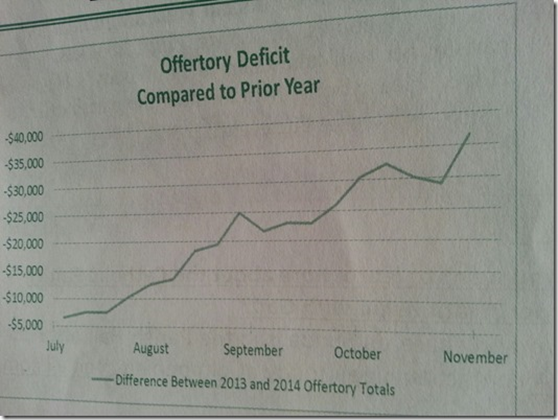
Visually Display Composite Data How To Create An Excel Waterfall Chart Pryor Learning Solutions

How To Move Chart X Axis Below Negative Values Zero Bottom In Excel

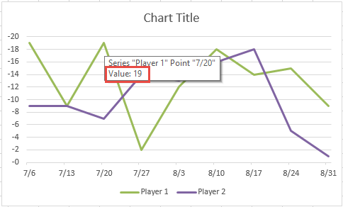
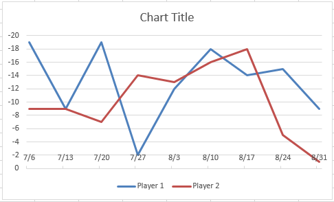
Best Excel Tutorial Chart With Negative Values
How To Make An Excel Chart Go Up With Negative Values Excel Dashboard Templates

Best Excel Tutorial Chart With Negative Values

Best Excel Tutorial Chart With Negative Values
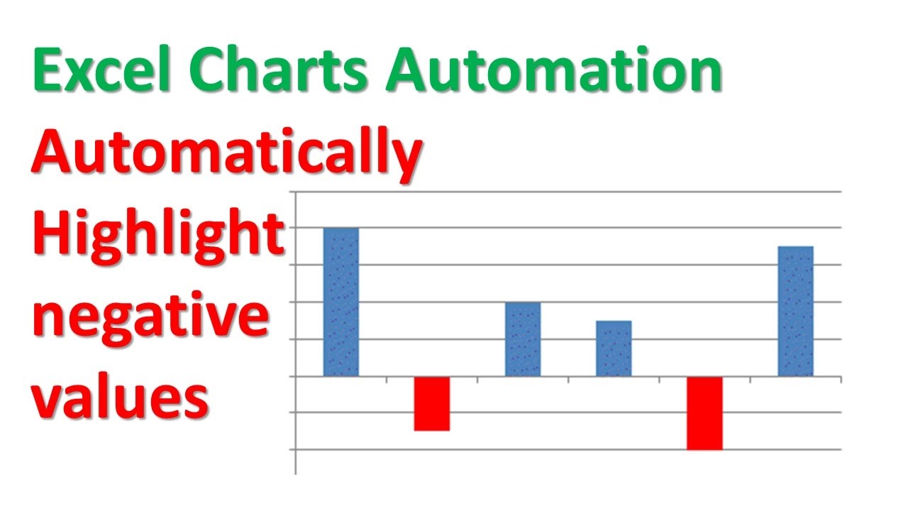
Excel Charts Automatically Highlight Negative Values Youtube
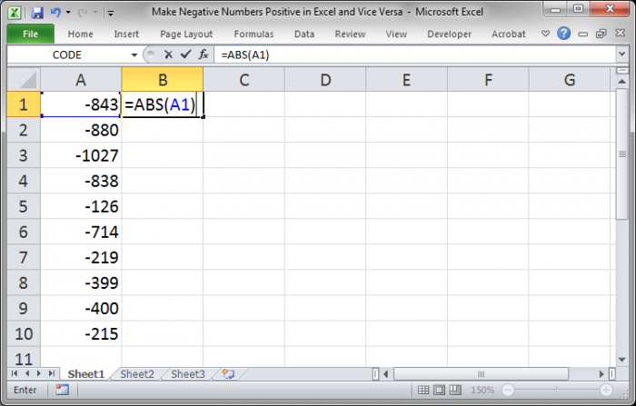
Make Negative Numbers Positive In Excel And Vice Versa Teachexcel Com

Best Excel Tutorial Chart With Negative Values
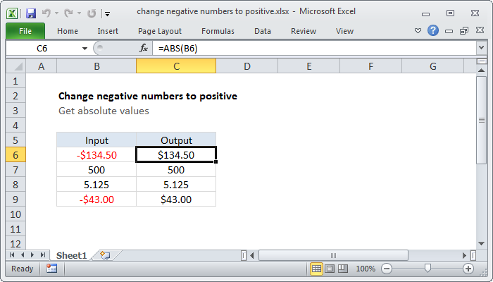
Excel Formula Change Negative Numbers To Positive Exceljet
How To Prevent Excel Charts From Displaying Negative Numbers Quora
How To Make An Excel Chart Go Up With Negative Values Excel Dashboard Templates

How To Plot Negative Numbers In Y Axis In Excel 2013 Super User

Formatting A Negative Number With Parentheses In Microsoft Excel
Excel Tip Make Number Negative Convert Positive Number To Negative Youtube